
Required: Pre-Flight Training – Spectra: SDSS Spectrum Graphs
Recommended: Pre-Flight Training – Redshift: The Basics
With some basic understanding about redshift and the tool of the SDSS spectrum graph in hand, you are prepared to explore how redshift is measured and how it can be used. We will need lots of spectra.
Accessing Data through the Science Archive Server (SAS)
If you want to look at a lot of spectra at one time, the easiest place to access them is through the Science Archive Server (SAS). SAS is the latest image and spectrum service for the SDSS. But before you can use SAS, you need a starting place.
 Space is vast and infinite, and with 500 million stars in the SDSS database, there are enough stars to go around for all researchers. Everyone should be able to start in a unique location, or Special Place (as you proceed in your experimentation and data collection, you will be able to build upon your knowledge base for your Special Place since you will continue to revisit it in other activities). If you completed the activity, My Special Place in the Database, you already have a set of coordinates as your own Special Place. Use the RA and Dec that you recorded during that activity. If you do not yet have your own Special Place, you will use RA and Dec to define a starting place (which will then become your Special Place, your very own “little plot of space real estate” to explore evermore).
If you already have a Special Place in the Database, great. Start there. If you don’t or need additional help to locate a starting place, you can choose one using the Constellations Notebook.
Working in SAS
When you arrive at an SAS Spectra List page, bookmark the location. Next, notice that each row represents a different object that was captured by the spectrograph. The Survey, Plate ID, and MJD columns are identical. This set of data was gathered under the same observing goals (Survey) using the same spectroscopic plate (Plate) on the same day (MJD). It isn’t until you get to the fourth column (Fiber #) that the information becomes unique. Scroll down and notice that there are either 640 or 1000 objects in the list depending upon the survey. You can reorder any column by clicking the up-down arrows on the column heading.
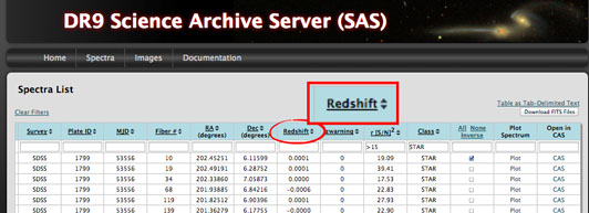
Launching into an exploration of redshift requires that we observe several different types of spectra. We can use the top row on the spectra list in SAS to sort the columns using a variety of commands. If you are familiar with SAS, sort your table to display stellar spectra with a signal-to-noise ratio greater than 15, ordered by increasing redshift. Follow the instructions below if you need help.
- Begin at your starting place in SAS
- Select objects that have less jagged spectral graphs by typing “>15” in the signal-to-noise ratio column – r(s/N)2
- Narrow your table to display only stars by typing STAR in the Class column
- Click the Redshift column header to sort the column in ascending order
Note the range of redshifts in the table.
What does zero redshift look like?
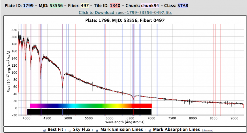
With your collection of stellar spectra at hand, locate a star with zero redshift. Clicking the plot link (or anywhere in the row, for that matter) opens the interactive spectrum tool. There can be a lot of different shapes for the continuum of a star. This activity is not concerned with the shape of the graphed line, so it doesn’t matter which stellar spectrum you pick. For now, focus on the bumps and dips (absorption and emission lines). Recall that the graph is the combination of the individual contributions of light from many different kinds of atoms.
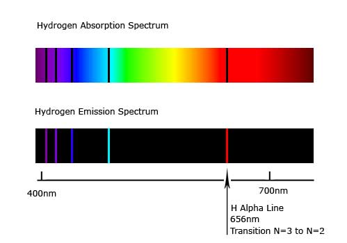

We begin by focusing on the pattern of light produced by hydrogen atoms (see image on left). Take note of any patterns you see or other features you are curious about. It’s likely there is an activity or resource in Voyages to help you explore further.
With your zero redshift spectrum in view, investigate the location of some of the absorption lines on your graph. The basic steps are listed below. Use the image below for a little help.
- Locate the wavelength of the Hydrogen Alpha line on the Line Measurement Information table in the Rest Wavelength column. Record that number.
- Locate the same line on the graph. If the redshift is zero, it should be in the same location reported. Later, this will not be as easy, so practice now. Do the numbers match exactly? Describe what you observe.
Find Redshifted Spectral Lines
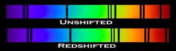
Astronomers determine redshift by locating patterns in the absorption or emission lines in a spectrum. They determine the amount the pattern is shifted from the standard that is produced in the laboratory as seen in the image below.
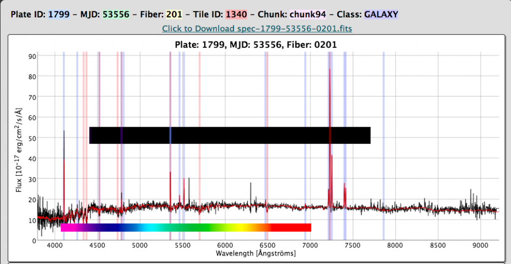
- Open a spectrum in the interactive tool
- Locate the familiar hydrogen alpha line. Record its location on the x-axis
- Observe several different galaxies with different redshifts. What else do you notice about the list of spectral lines recorded for each galaxy?
Remember, the range of wavelengths your eye sees remains the same. Only the position of individual spectral lines changes.
Calculate Redshift
We use the observed position of a known absorption or emission line and the position where we would expect to find the feature with no redshift (rest wavelength in SDSS) to calculate a value for redshift that compared.
z = (λobserved – λrest) / λrest
Using what you know about SAS spectrum plots, demonstrate this calculation for one galaxy.
The SDSS Filters and Redshift
Just as the portion of the electromagnetic spectrum that our eyes see does not change, so are the SDSS filters fixed with respect to the spectrum. However, the amount (flux) of light that is captured in each of the filters does change with increased redshift. The simulation below demonstrates this. Observe the changes in the continuum of the spectrum as well as the nature of the light transmitted by each filter. Record these observations.